Estimate RRi Curve Using a Dual-Logistic Model for RR Interval Dynamics (Castillo-Aguilar et al.)

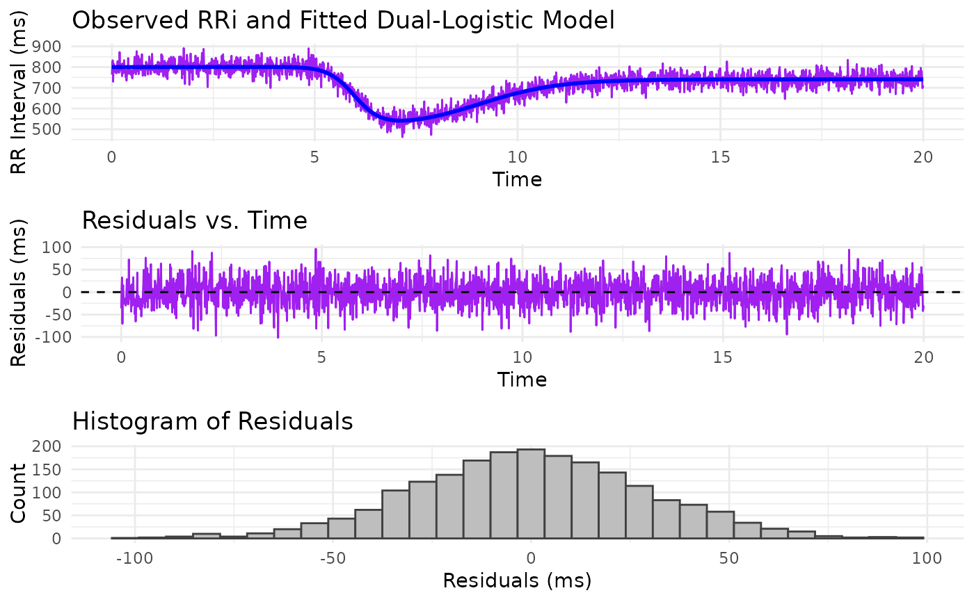
This function estimates parameters for a dual-logistic model applied to RR interval (RRi) signals. The model is designed to capture both the rapid drop and subsequent recovery of RRi values during exercise and recovery periods, as described in Castillo-Aguilar et al. (2025). A robust Huber loss function (with a default $\delta$ of 50 ms) is used to downweight the influence of outliers, ensuring that the optimization process is robust even in the presence of noisy or ectopic beats.

Usage

estimate_RRi_curve(
  time,
  RRi,
  start_params = c(alpha = 800, beta = -380, c = 0.85, lambda = -3, phi = -2, tau = 6,
    delta = 3),
  lower_lim = c(alpha = 300, beta = -750, c = 0.1, lambda = -10, phi = -10, tau =
    min(time), delta = min(time)),
  upper_lim = c(alpha = 2000, beta = -10, c = 2, lambda = -0.1, phi = -0.1, tau =
    max(time), delta = max(time)),
  method = "L-BFGS-B"
)

Arguments

time: A numeric vector of time points.
RRi: A numeric vector of RR interval values.
start_params: A named numeric vector or list of initial parameter estimates. Default is c(alpha = 800, beta = -380, c = 0.85, lambda = -3, phi = -2, tau = 6, delta = 3).
lower_lim: A named numeric vector specifying the lower bound for each parameter. Default is c(alpha = 300, beta = -750, c = 0.1, lambda = -10, phi = -10, tau = min(time), delta = min(time)).
upper_lim: A named numeric vector specifying the upper bound for each parameter. Default is c(alpha = 2000, beta = -10, c = 2.0, lambda = -0.1, phi = -0.1, tau = max(time), delta = max(time)).
method: A character string specifying the optimization method to use with optim(). The default is "L-BFGS-B", which allows for parameter constraints.

Value

A list containing:

data: A data frame with columns for time, the original RRi values, and the fitted values obtained from the dual-logistic model.
method: The optimization method used.
parameters: The estimated parameters from the model.
objective_value: The final value of the objective (Huber loss) function.
convergence: An integer code indicating convergence (0 indicates success).

Details

The dual-logistic model, as described in Castillo-Aguilar et al. (2025), is defined as:

$$ RRi(t) = \alpha + \frac{\beta}{1 + e^{\lambda (t - \tau)}} + \frac{-c \cdot \beta}{1 + e^{\phi (t - \tau - \delta)}} $$

where:

$\alpha$: is the baseline RRi level.
$\beta$: controls the amplitude of the drop.
$\lambda$: modulates the steepness of the drop phase.
$\tau$: represents the time at which the drop is centered.
$c$: scales the amplitude of the recovery relative to $\beta$.
$\phi$: controls the steepness of the recovery phase.
$\delta$: shifts the recovery phase in time relative to $\tau$.

The function first removes any missing cases from the input data and then defines the dual-logistic model, which represents the dynamic behavior of RR intervals during exercise and recovery. The objective function is based on the Huber loss (with a default threshold of 50 ms), which provides robustness against outliers by penalizing large deviations less harshly than the standard squared error. This objective function quantifies the discrepancy between the observed RRi values and those predicted by the model.

Parameter optimization is performed using optim() with box constraints when the "L-BFGS-B" method is used. These constraints ensure that the parameters remain within physiologically plausible ranges. For other optimization methods, the bounds are ignored by setting the lower limit to -Inf and the upper limit to Inf.

It is important to note that the default starting parameters and bounds provided in the function are general guidelines and may not be optimal for every dataset or experimental scenario. Users are encouraged to customize the starting parameters (start_params) and, if necessary, the lower and upper bounds (lower_lim and upper_lim) based on the specific characteristics of their RRi signal. This customization is crucial for achieving robust convergence and accurate parameter estimates in diverse applications.

References

Castillo-Aguilar, et al. (2025). Enhancing Cardiovascular Monitoring: A Non-linear Model for Characterizing RR Interval Fluctuations in Exercise and Recovery. Scientific Reports, 15(1), 8628.

Examples

true_params <- c(alpha = 800, beta = -300, c = 0.80,
                 lambda = -3, phi = -1, tau = 6, delta = 3)

time_vec <- seq(0, 20, by = 0.01)

set.seed(1234)

# Simulate an example RRi signal:
RRi_simulated <- dual_logistic(time_vec, true_params) +
                  rnorm(length(time_vec), sd = 30)

# Estimate the model parameters:
fit <- estimate_RRi_curve(time = time_vec, RRi = RRi_simulated)

# Print method
print(fit)
#> RRi_fit Object
#> Optimization Method: L-BFGS-B 
#> Estimated Parameters:
#>        alpha         beta            c       lambda          phi          tau 
#>  800.0103101 -295.1123155    0.7991941   -3.0636912   -1.0268231    5.9785596 
#>        delta 
#>    3.1004798 
#> Objective Value (Huber loss): 852819.5 
#> Convergence Code: 0 

# Summary method
summary(fit)
#> Summary of RRi_fit Object
#> Optimization Method: L-BFGS-B 
#> Estimated Parameters:
#>        alpha         beta            c       lambda          phi          tau 
#>  800.0103101 -295.1123155    0.7991941   -3.0636912   -1.0268231    5.9785596 
#>        delta 
#>    3.1004798 
#> 
#> Objective Value (Huber loss): 852819.5 
#> Residual Sum of Squares (RSS): 1758802 
#> Total Sum of Squares (TSS): 12795299 
#> R-squared: 0.8625 
#> Root Mean Squared Error (RMSE): 29.6  ms 
#> Mean Absolute Percentage Error (MAPE): 3.3  % 
#> Number of observations: 2001 
#> Convergence Code: 0 

# Plot method
plot(fit)